
How to Calibrate Your LVDTs
Written by transtek_admin on 06/28/2022
Calibration of your LVDT’s is critical to ensure that they are operating within the tolerances of precision and accuracy for which they are well known. That is why every sensor that leaves our factory is calibrated prior to shipping. Today we will detail the approach that we use, along with the information that is included with our reports. While other methods may vary a bit, we’ve found this one to be most accurate and effective. We hope you find this as a useful tool for guiding your own calibration efforts.
You start by establishing and recording the reference data. This process starts by electrically exciting the transducer then mechanically setting the transducer at its null position. You’ll then record the output voltage. Data should be taken at both positive and negative points, and other positions in between. The next step is to compare the collected data to the allowable values. Keep in mind that values will vary from model to model, so be sure to have the manufacturer’s stated values handy. Here are the attributes and calculations that are required for testing and reporting, following our standard reporting format:
Maximum Non-Linearity – This is the greatest absolute difference between the transducer’s output and the calculated line, expressed as a percentage of full scale. We’ll take a look at the calculations in a moment in the Calibration Data section.
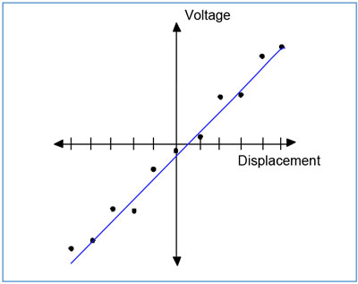
Calculation Method – The data taken is compared to a calculated line which is assumed to represent an ideal transducer. There are approaches you can use as follows:
- Zero Base – Average Terminal – this is a somewhat rudimentary approach which is simple enough to calculate manually. Data is taken over the measurement range. To force a line between the measured endpoints through zero, a new line is generated by taking the average value of the existing endpoints. Each data point is compared against this line, and non-linearity is computed.
- Best Fit Straight Line – Unlike the previous method, this one is calculation intensive that requires a computer to analyze the data. Data taken from a transducer is analyzed numerically to produce a line which minimizes the worst non-linearity at any given point in the line.
- Best Fit Straight Line Through Zero – In order to calculate an ideal line with this approach, the line must have a y-intercept of zero. The slope of this line is adjusted around the zero point until the resulting non-linearity at each point is at its lowest value.
Calculated Line – Here, you finally get to apply a formula you likely learned in high school geometry: y=mX+b. In this real life application of the equation, you calculate theoretically output at a specific position by substituting a displacement for X.
Working Range – This represents the total range which the transducer was calibrated. For certain units, manufacturers will provide both a linear range and maximum usable range. For most cases, the calibration should be performed over the specified linear range.
Sensitivity – This indicates the relationship between the position measured and the voltage output expressed in units of Volts Output/Unit Displacement/Volts Input. It is calculated by the slope (m) of the calculated line divided by the voltage input.
Tested At – This is used to determine the sensitivity of the transducer. It represents the voltage at which the calibration data was collected. For DC transducers, voltage and minimum load impedance are relevant. For AC sensors, RMS voltage and frequency are relevant.
Calibration Data – Here, you are showing the data taken during calibration, focusing on the numbers used to calculate the maximum non-linearity, as we discussed early in this article. Key data points include:
- Position – the mechanical position in which the data was taken
- Data – the actual output voltage at each position
- Zero Adjust Data – for DC sensors, the voltage at zero displacement is not always 0.0000 VDC resulting in residual voltage, known as zero offset, which needs to be compensated for. The zero adjust data is the output voltage at each position minus residual null voltage.
It’s important to note that AC LVDTs must be calibrated a little differently, due to their quadrature voltage. Rather than set the unit to operate at 0.0000 volt null position, the AC LVDT’s data is taken symmetrically around the point of lowest RMS output. The residual quadrature voltage is the out-of-phase component, which is removed by demodulation.
Error % F.S.
To establish non-linearity at each point, you will first subtract the zero adjusted output from the calculated value at each point. The difference is then divided by the full scale voltage swing of the calculator line. Multiply this number by 100 to get the percentage. The largest absolute value found represents the maximum non-linearity for the unit.